c. Single-cell RNA-Seq data
Bulk RNA sequencing allows researchers to discern the average gene expression profiles of their samples of interest, but the results are limited in their resolution, and affected by variation in cell type composition. The application of microfluidics and / or multi-step barcoding strategies to molecular biology along with advances in next-generation sequencing technologies have allowed researchers to utilise single cell technologies, such as droplet-based and combinatorial barcoding approaches, at a high-throughput scale. Single cell measurements complement bulk RNA sequencing profiles by allowing for granular insights into gene expression and gene regulatory networks, and facilitating an understanding of cell type composition and cell-to-cell heterogeneity in samples of interest.
In this introductory session on Day 1 of the GIS-AWS training, we will explore the data and metadata structure of a single cell dataset. This exercise features a single cell dataset that we have pre-processed using Seurat, one of the most popular single cell analysis R packages. Today, we will get familiarised with using R in the AWS EC2 environment. On Day 2 of the GIS-AWS training, we will identify major cell types present in this single cell dataset.
First, let’s make a directory for this exercise and download some data:
mkdir -p /tmp/SingleCell
cd /tmp/SingleCell

aws s3 cp s3://gisxaws-training/pbmc3k_final_withoutRCA2.rds .
The analysis is run with the installation of R from the Chen lab AMI, which includes multiple R packages useful for single cell analysis. Start up the R environment:
R
Then, we will load our libraries and data file:
library(dplyr)
library(Seurat)

data <- readRDS(file = "pbmc3k_final_withoutRCA2.rds")
We will analyse this dataset on Day 2, but for now familiarise yourself with navigating in R. R allows users to perform statistical analyses and data visualisation. There is a graphic user interface known as RStudio, but for this workshop we will be the R terminal interface only.
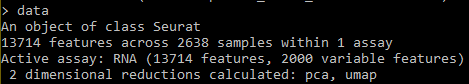
- Examine the data object: data is a pre-processed Seurat object and contains a gene-cell matrix, along with metadata and quality control (QC) metrics for each cell. How many genes and cells are there in this pre-processed dataset?
data
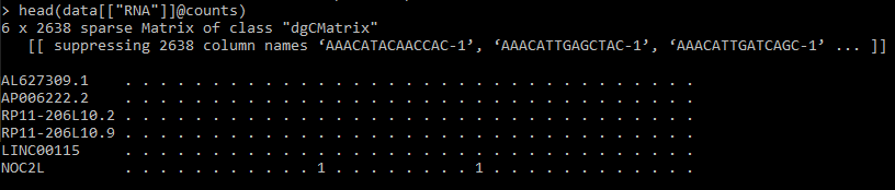
 2. Examine the gene-cell matrix containing the raw counts.
head(data[["RNA"]]@counts)
Each row corresponds to a specific gene (“feature”), and each column corresponds to a specific cell (“sample”). This gene-cell matrix takes the form of a sparse matrix (where “0"s are represented by “.") for optimising memory usage and computational speed.
3. Examine the metadata and QC metrics for each cell.
head(data)
Each row corresponds to a specific cell (“sample”).
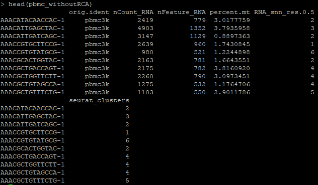
There are several QC metrics in this pre-processed Seurat object, including:
nCount_RNA -> The number of unique molecular identifiers (UMIs, corresponding to the number of unique molecules) detected within a single cell
nFeature_RNA -> The number of detected genes within a single cell
percent.mt -> Percentage of mitochondrial UMIs out of the total UMIs in a cell
For a sample single cell gene expression pre-processing workflow, please see the Seurat Guided Clustering Tutorial from the Satija Lab. For more details on interacting with Seurat objects, please see the documentation of essential Seurat R package commands.