Add'l-3: RNA-Seq data-Bambu
Usage examples of Bambu
In this tutorial we will be using human cancer cell-line data from the SG-NEx project. In total we will use 6 direct RNA Nanopore long-read samples, 3 replicates each from the A549 and HepG2 cell lines. The A549 cell line was extracted from lung tissues from a patient with lung cancer. HepG2 was extracted from hepatocellular carcinoma from a patient with liver cancer. We will use Bambu to identify and quantify novel isoforms in these two cell lines.
Downloading reference genome and annotations
As mentioned in #Bambu-Day 1, the default mode to run Bambu is using a set of aligned reads (bam files), reference genome annotations (gtf file, TxDb object, or bambuAnnotation object), and reference genome sequence (fasta file or BSgenome). Here we use the ensembl GRCh 38 genome sequence and annotation files, which we have downloaded and stored in the SG-NEx data open S3 bucket.
# create working directory
mkdir /home/ubuntu/bambu_training
cd /home/ubuntu/bambu_training

# download genome fasta file
aws s3 cp --no-sign-request s3://sg-nex-data/data/annotations/genome_fasta/Homo_sapiens.GRCh38.dna_sm.primary_assembly.fa ./
aws s3 cp --no-sign-request s3://sg-nex-data/data/annotations/genome_fasta/Homo_sapiens.GRCh38.dna_sm.primary_assembly.fa.fai ./

# download gtf file
aws s3 cp --no-sign-request s3://sg-nex-data/data/annotations/gtf_file/Homo_sapiens.GRCh38.91.gtf ./
Downloading and aligning reads
The SG-NEx project provides aligned reads that can be used directly with Bambu, however sometimes, raw fastq reads might be provided instead of aligned reads. In that case, alignment must be done first and can be done as follows:
Note that we are aligning the reads to the genome fasta and not the transcriptome fasta as Bambu uses intron junctions to distinguish novel transcripts.
# download fastq from s3 bucket
aws s3 cp --no-sign-request s3://sg-nex-data/data/data_tutorial/fastq/A549_directRNA_sample1.fastq.gz ./

# align using Minimap2 - note this step needs more than 8GB of RAM, otherwise it will get killed automatically after a minute or so
minimap2 -ax splice -uf -k14 Homo_sapiens.GRCh38.dna_sm.primary_assembly.fa A549_directRNA_sample1.fastq.gz > A549_directRNA_sample1.sam
samtools view -Sb A549_directRNA_sample1.sam | samtools sort -o A549_directRNA_sample1.bam
samtools index A549_directRNA_sample1.bam
For this analysis, you can directly download the bam files needed from the open S3 bucket
# download aligned bam files for A549 samples and a pre-processed se (summarizedExperiment) object
aws s3 sync --no-sign-request s3://sg-nex-data/data/data_tutorial/bam/ ./ --exclude "*" --include "A549_directRNA*"
aws s3 cp --no-sign-request s3://sg-nex-data/data/data_tutorial/bam/se.rds ./
Quality Control
Samtools stats can be used to quickly check the read accuracy and read mappability in the bam files, in the example below, we checked the aligned bam file for the SGNex_A549_directRNA_replicate1_run1 sample.
# quickly check the number of reads mapped in the bam file, and also read accuracy
samtools stats A549_directRNA_sample1.bam | head -46
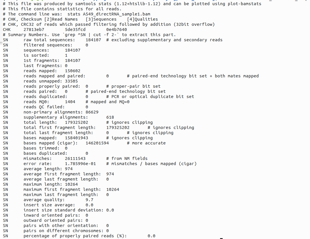
This bam file has a read mappability of 150602/184107 (81.8%) by taking the ratio between reads mapped and raw total sequences and a read accuracy of 1-0.178599 (0.821%) by minusing 1 with the error rate. Usually we consider a sample with a mappability of 80% above as relatively good, and the read accuracy is also common for Nanopore reads.
Preparing data for Bambu
R

# set work directory
setwd("bambu_training") #if you are in a different directory


library(bambu)
fa.file <- "Homo_sapiens.GRCh38.dna_sm.primary_assembly.fa"
gtf.file <- "Homo_sapiens.GRCh38.91.gtf"
annotations <- prepareAnnotations(gtf.file) # this will prepare annotation object for Bambu, gtf file can be loaded directly, but for best practice, you can create annotation object first, and then you can use it repeatedly with Bambu without the need to prepare it again.


samples.bam <- list.files(".", pattern = ".bam$", full.names = TRUE)
Running Bambu
To run Bambu is using, you will need
- a set of aligned reads (bam files),
- reference genome annotations (gtf file, TxDb object, or bambuAnnotation object),
- and reference genome sequence (fasta file or BSgenome).
Bambu will return a summarizedExperiment object with
- the genomic coordinates for annotated and new transcripts
- and transcript expression estimates.
We highly recommend to use the same annotations that were used for genome alignment.
Running bambu with this data will take about 5-10 mins to run. Therefore we will skip this step and load in the result. Below is the line we used so you can run it later in your free time.
dir.create("./rc")
# se <- bambu(reads = samples.bam, annotations = annotations, genome = fa.file, rcOutDir = "./rc")
As we used the rcOutDir argument with Bambu the read class files were automatically saved, allowing us to restart transcript discovery or quantification. For more details please see the Bambu documentation.
To load in the pre-processed data we prepared earlier.
# you can just load pre-saved se object
se <- readRDS("./se.rds")
Output
Bambu returns a SummarizedExperiment object which can be accessed as follows:
assays(se) #returns the transcript abundance estimates as counts or CPM
rowRanges(se) #returns a GRangesList with all annotated and newly discovered transcripts
rowData(se) #returns additional information about each transcript such as the gene name and the class of newly discovered transcript
Write output
The output can be written to files:
writeBambuOutput(se, path = "./")
The above command will write Bambu output to three files
- extended_annotations.gtf
- counts_transcripts.txt
- counts_gene.txt
The .gtf format is used by bioinformatic tools to describe the location of genomic features, such as genes. Below is how to output the newly discovered annotations from Bambu as a .gtf for use in downstream tools. Keep in mind that the novel annotations are added to the reference annotations, so all original annotations will still be present in the output. To remove the known annotations, filtering needs to be done and will be shown in a later step.
Gene and transcript expression are also output to a txt file.
Identify novel transcripts in one sample and not another
Now let’s find some novel transcripts that occur uniquely in A549 but not in HepG2 and visualise them. First we will filter the annotations to remove the reference annotations. Then we can sort them by the txNDR, which ranks them by how likely they are a real transcript.
se.filtered <- se[mcols(rowRanges(se))$newTxClass != "annotation",]
#investigate high confidence novel isoforms
head(mcols(rowRanges(se.filtered))[order(mcols(rowRanges(se.filtered))$txNDR),])
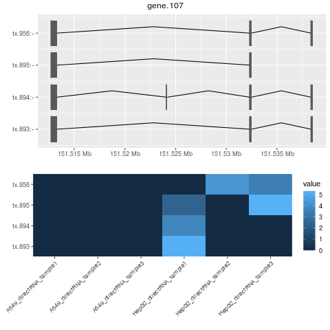
png("gene.107.png")
plotBambu(se, type = "annotation", gene_id = "gene.107")
dev.off()
#no novel genes
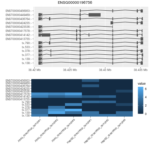
se.filtered.noNovelGene = se.filtered[rowData(se.filtered)$newTxClass != "newGene-spliced",]
head(mcols(rowRanges(se.filtered.noNovelGene))[order(mcols(rowRanges(se.filtered.noNovelGene))$txNDR),])
png("ENSG00000196756.png")
plotBambu(se, type = "annotation", gene_id = "ENSG00000196756")
dev.off()
#find which ones are unique based on counts
expression.A549 <- apply(assays(se.filtered)$counts[,grep("A549",colnames(se.filtered))],1,mean)
expression.HepG2 <- apply(assays(se.filtered)$counts[,grep("HepG2",colnames(se.filtered))],1,mean)


se.filtered[expression.A549>=1 &(expression.HepG2==0)] # unique in A549
se.filtered[expression.A549==0 &(expression.HepG2>=1)] # unique in HepG2
If you have tex installed, then you can directly visualize with the plotBambu command. However, if you don’t have tex pre-installed, then you can follow the commands above to generate the png first and then upload them to the S3 bukcet for visualization.
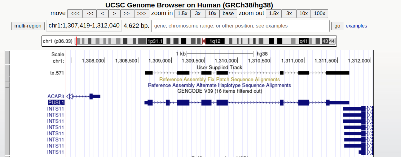
UCSC genome browser
We can visualise these novel transcripts using a genome browser such as IGV or the UCSC genome browser. For this tutorial we will use the UCSC genome browser.
First we need to produce the bed files from the new transcripts:
annotations.UCSC = rowRanges(se.filtered)
seqlevelsStyle(annotations.UCSC) <- "UCSC" #this reformats the chromosome names
annotations.UCSC = keepStandardChromosomes(annotations.UCSC, pruning.mode="coarse") #removes chromosomes UCSC doesn't have
writeToGTF(annotations.UCSC, "./novel_annotations.UCSC.gtf")
q()
n
Now we can upload the annotations created to the public accessible bucket that we have created before in Section XIIc-Step 12. We will need to manage access to the object using the access control lists (ACLs).
aws s3 cp novel_annotations.UCSC.gtf s3://bucket/path/ --acl public-read
Now go to https://genome.ucsc.edu/ in your browser
My data > Custom Tracks > add custom tracks
In the box labeled “Paste URLs or data” copy in path of the file you copied onto your bucket
To obtain the S3 URL of the object in the S3 bucket
-Click on the object name in the S3 bucket (here “novel_annotations.UCSC.gtf”)
-Copy the link under “Object URL”
Remember to verify the correct “bucket” name and the “path”
https://“bucket”.s3.ap-southeast-1.amazonaws.com/“path”/novel_annotations.UCSC.gtf